Partial Differentiation
Earlier in the year we learned how to differentiate a function.Today we took that a step further by talking about PARTIAL DIFFERENTIATION!!! Basically, partial differentiation is the process of finding the derivative in regards to a single term–either x or y. This process can be used when a function has more than one variable. Before we can take the partial derivative of a function, we need to learn about some new notation. denotes that a function is in terms of both the x and y
 denotes that a partial derivative needs to be taken in terms of x
 denotes that a partial derivative needs to be taken in terms of y
denotes that a function is in terms of both the x and y denotes that a partial derivative needs to be taken in terms of x denotes that a partial derivative needs to be taken in terms of y
Likewise, the partial derivative notations above can be written as  and
and  or as
or as  and
and  .
.
and or as and .
For the majority of first and second semester we used limit definitions to understand how and why derivatives work. Even though limits are not the most efficient way to find derivatives, they’re important when understanding them fully. Remember that derivatives have a limit definition of  . The definition of a partial derivative using limits can be split into both an x and a y component, but both follow the basic structure of the original limit definition. However, each variable is approaching a separate number. As h approaches zero, x approaches a and y approaches b. This is written as:
. The definition of a partial derivative using limits can be split into both an x and a y component, but both follow the basic structure of the original limit definition. However, each variable is approaching a separate number. As h approaches zero, x approaches a and y approaches b. This is written as: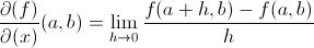 and
and 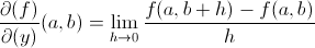
Notice, that in the numerator, h is placed with a, since that is the value x is approaching. Likewise, when taking the partial derivative of y, h is placed with b, since that is the value that y is approaching. Basically what the limit definition explains is that partial differentiation requires that you only take the derivative with regards to one variable at a time and leave the other as a constant. That really is the most important thing to keep in mind when finding partial derivatives. ALWAYS treat the variable that you’re NOT taking the partial derivative of as a constant. For example... 


Before getting into higher order partial derivatives, it’s also important to understand the geometric representation of a partial derivatives. In this case we’re looking at a three-dimensional surface, in the x, y, z axes. Just as the derivative of a function represents the slope of a tangent line to  at
at  ,
,  and
and  are the slopes of tangents lines. However, there’s a difference. They are slopes of traces of surfaces, which are curves that represent the intersection of the surface and the plane given by
  or
or  . That is, when taking the derivative in terms of y, it is the slope of the tangent plane in the y direction. Likewise, the derivative in terms of x represents the slope of the tangent plane in the x direction. Later, as we talk about higher order partial derivatives, you’ll see that when you take a derivative in terms of both x and y, it’s geometric representation can be described as the rate of change of the slope in the x-direction as one moves in the y-direction. In order to understand these concepts more clearly, this applet will be helpful.
at , and are the slopes of tangents lines. However, there’s a difference. They are slopes of traces of surfaces, which are curves that represent the intersection of the surface and the plane given by or . That is, when taking the derivative in terms of y, it is the slope of the tangent plane in the y direction. Likewise, the derivative in terms of x represents the slope of the tangent plane in the x direction. Later, as we talk about higher order partial derivatives, you’ll see that when you take a derivative in terms of both x and y, it’s geometric representation can be described as the rate of change of the slope in the x-direction as one moves in the y-direction. In order to understand these concepts more clearly, this applet will be helpful.
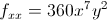
Taking higher order partial derivatives is relatively easy. You simply take the partial derivative in terms of either x or y, and then take the partial derivative in terms of x or y again, depending on the problem. Here’s an example:


Just like there were differentials for functions with one variable, there are also differentials for functions with multiple variables. We learned this year that differentials were: 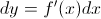
With multiple variables, this becomes written as: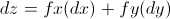
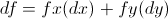
Those two differential equations above are synonymous. What this is saying is that the differential of a function with two variables is just equal to the sum of the partial derivative of x and y multiplied by a change in x and change in y respectively. This can likewise be expanded if you had a function with more than two variables, such as  :
:
:
If you’re still feeling a bit stuck, here are two PatrickJMT videos to refer to!
No comments:
Post a Comment